Does Luke turn to the Dark Side?
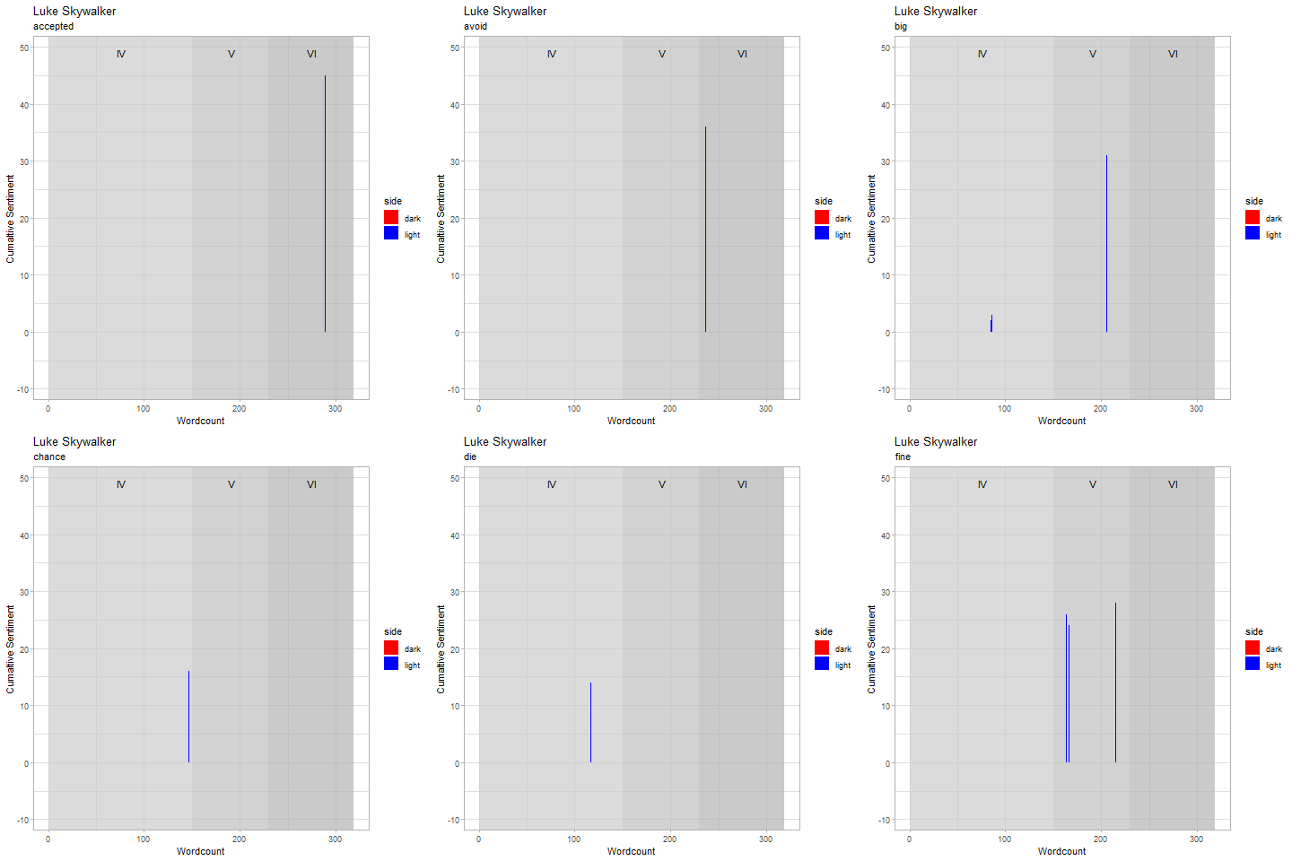
A few weeks ago I attended a text analytics hackathon, that was immensely enjoyable. Text analysis is something that is quite far from my average day job and I really enjoyed picking up some new skills and playing with the tidytext package. If you are looking to dive into text analytics, I thoroughly recommend the brilliant Text Mining with R book by Julia Silge and David Robinson. The data we experimented with at the event was the three scripts from THE Star Wars Trilogy (you know which one I mean) and I was keen to see if we could use sentiment analysis to distinguish whether a character was from the Light or Dark side. Additionally I wanted to see if we could track a character’s journey through the 3 films and see how their sentiment fluctuated.
So lets load up our packages.
library(tidyverse)
library(tidytext)
library(gganimate)
library(magick)
Luckily for us the data exists on GitHub, which helps us read the data straight into R.
## Url for each film's script
urls <- c("https://raw.githubusercontent.com/gastonstat/StarWars/master/Text_files/SW_EpisodeIV.txt",
          "https://raw.githubusercontent.com/gastonstat/StarWars/master/Text_files/SW_EpisodeV.txt",
          "https://raw.githubusercontent.com/gastonstat/StarWars/master/Text_files/SW_EpisodeVI.txt")

## Read in each script and combine them into one dataframe. Ensure each film is marked by the Episode numeral.
raw_data <-
  map_dfr(urls, read.table, .id = "film") %>%
  mutate(film = recode(film, `1` = "IV", `2` = "V", `3` = "VI"))

head(raw_data)
##   film character
## 1   IV  THREEPIO
## 2   IV  THREEPIO
## 3   IV  THREEPIO
## 4   IV  THREEPIO
## 5   IV  THREEPIO
## 6   IV      LUKE
##                                                                                                   dialogue
## 1  Did you hear that?  They've shut down the main reactor.  We'll be destroyed for sure.  This is madness!
## 2                                                                                            We're doomed!
## 3                                                        There'll be no escape for the Princess this time.
## 4                                                                                             What's that?
## 5 I should have known better than to trust the logic of a half-sized thermocapsulary dehousing assister...
## 6                                       Hurry up!  Come with me!  What are you waiting for?!  Get in gear!
Now we have read the data in, we can see we have three columns, denoting the film, character speaking and their line of dialogue. Now the first part of this analysis is to split the dialogue into separate words, using the unnest_tokens function from the tidytext package.
words_per_char <-
  raw_data %>%
  unnest_tokens(word, dialogue)

head(words_per_char)
##     film character    word
## 1     IV  THREEPIO     did
## 1.1   IV  THREEPIO     you
## 1.2   IV  THREEPIO    hear
## 1.3   IV  THREEPIO    that
## 1.4   IV  THREEPIO they've
## 1.5   IV  THREEPIO    shut
Now we have the words by character we can visualise the most common words, spoken by the most important characters. The stop_words dataframe, combined with dplyr’s anti_join allows us to eliminate pesky stop words, such as “the” and “it”, so we can focus on words that can provide us with more insight.
Within this section of code you will see a reference to the drlib package. This is because I want to reorder the word column dependent upon the character. If I was to plot this using an average reorder, any character would have “Luke” as the top of their chart, because he was the most spoken word, even if that character didn’t say “Luke” much.
## Identify the 9 characters who speak the most words
top_9_chars <-
  words_per_char %>%
  count(character) %>%
  top_n(9) %>%
  select(character)

## Install David Robinsons package to get the reordering within a facet.
## devtools::install_github("dgrtwo/drlib")

words_per_char %>%
  count(character, word) %>%
  ## Remove the pesky stop words
  anti_join(stop_words) %>%
  ## Keep only the 9 characters with the most words
  inner_join(top_9_chars) %>%
  group_by(character) %>%
  ## Get the 10 most frequent words spoken by character
  top_n(10) %>%
  ggplot(aes(drlib::reorder_within(word, n, character), n, fill = character)) +
  drlib::scale_x_reordered() +
  geom_col() +
  facet_wrap(~character, scales = "free") +
  coord_flip() + guides(fill = F) +
  theme_light() +
  labs(title = "Most frequent words", subtitle = "By characters with the most words", x = "Word", y = "Number of times")
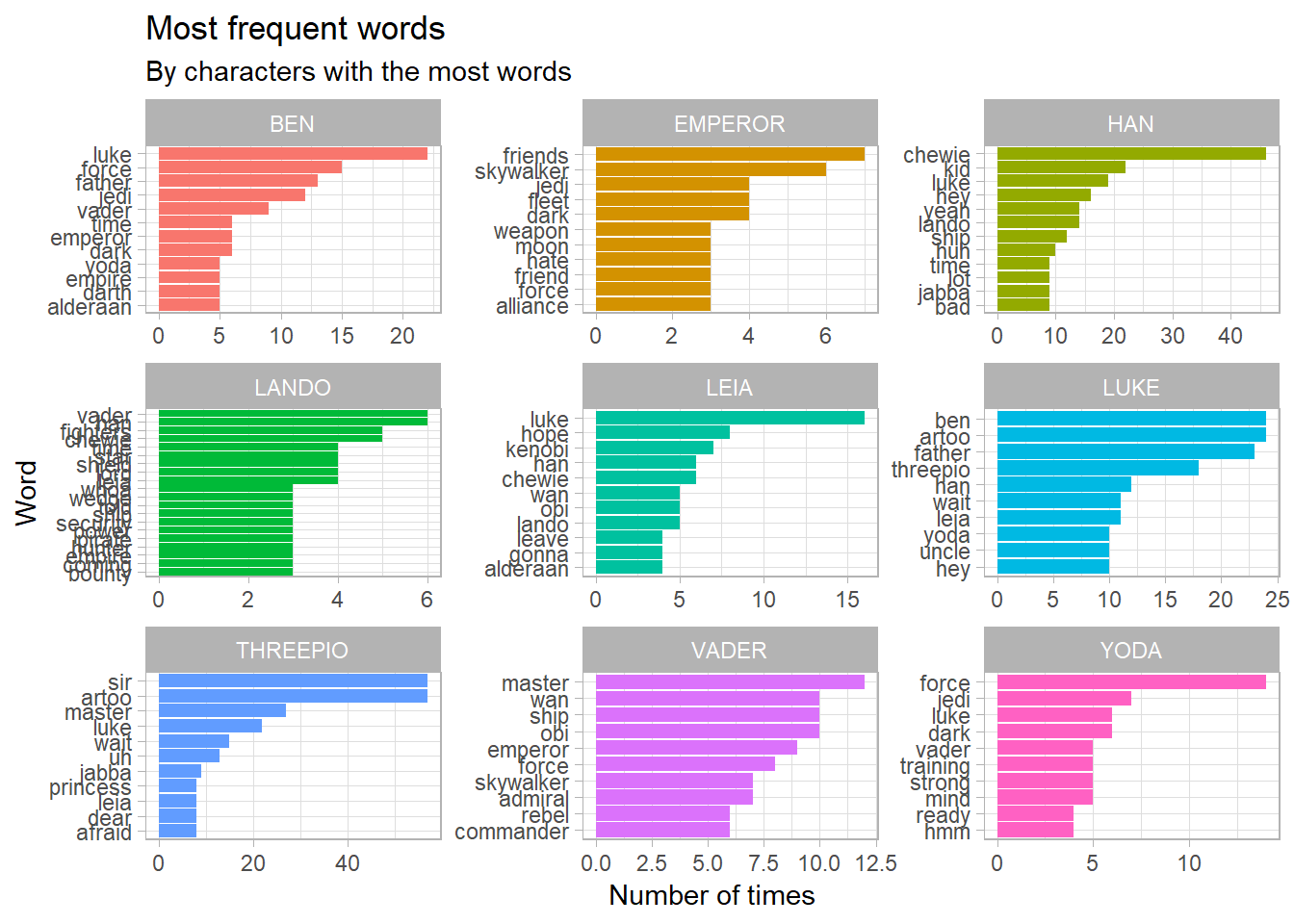
We can see some of the classic words coming out in this chart, the “sir” from Threepio and “master” from Darth Vader, with “Luke” seeing plenty of action.
Now let’s crack on with undertaking the sentiment analysis. The tidytext package comes with three built-in sentimnet lexicons:
AFINNlexicon, which assigns a score between -5 and 5, where negative numbers indicate negative sentiment and positive numbers indicating postitive sentiment.binglexicon, which categorises words in a binary fashion, either positive or negative.nrclexicon, which categorises words into a number of different categories, such as anger, disgust, surprise etc..
For this piece of analysis I decided to use the AFINN lexicon, so the more negative/positive a word is, the greater it will be scored. For this piece of analysis I’ve made the very broad assumption that words scored with a positive sentiment indicate the character is acting in “the Light side of the Force” and vice-versa.
word_sentiments <-
  words_per_char %>%
  ## Join on the sentiment score and keep only words that have been scored
  inner_join(get_sentiments("afinn")) %>%
  group_by(character) %>%
  mutate(wordcount = 1:n(),
         cuma_sent = cumsum(score),
         side = if_else(cuma_sent > 0, "light", "dark"),
         word_side = if_else(score > 0, "light", "dark"))
Now that we’ve assigned sentiment to the words used we can plot over time and see how this sentiment has fluctuated. So if we take Luke as an example:
minmax <-
  word_sentiments %>%
  filter(character == "LUKE") %>%
  group_by(film) %>%
  summarise(min = min(wordcount),
            max = max(wordcount))

word_sentiments %>%
  filter(character == "LUKE") %>%
ggplot() +
  labs(y = "Cumaltive Sentiment", x = "Wordcount", title = "Luke Skywalker") +
  theme_light() +
  geom_rect(alpha = 0.7, fill = "grey80", aes(xmin = 0, xmax = minmax$max[1], ymin = -Inf, ymax = Inf)) +
  geom_rect(alpha = 0.7, fill = "grey75", aes(xmin = minmax$min[2]-1, xmax = minmax$max[2], ymin = -Inf, ymax = Inf)) +
  geom_rect(alpha = 0.7, fill = "grey70", aes(xmin = minmax$min[3]-1, xmax = minmax$max[3]+1, ymin = -Inf, ymax = Inf)) +
  geom_col(aes(wordcount, cuma_sent, fill = side), width = 1.01) +
  geom_text(aes(x = (minmax$max[1] + minmax$min[1])/2, y = 50), label = "IV") +
  geom_text(aes(x = (minmax$max[2] + minmax$min[2])/2, y = 50), label = "V") +
  geom_text(aes(x = (minmax$max[3] + minmax$min[3])/2, y = 50), label = "VI") +
  scale_fill_manual(values = c("red", "blue"))
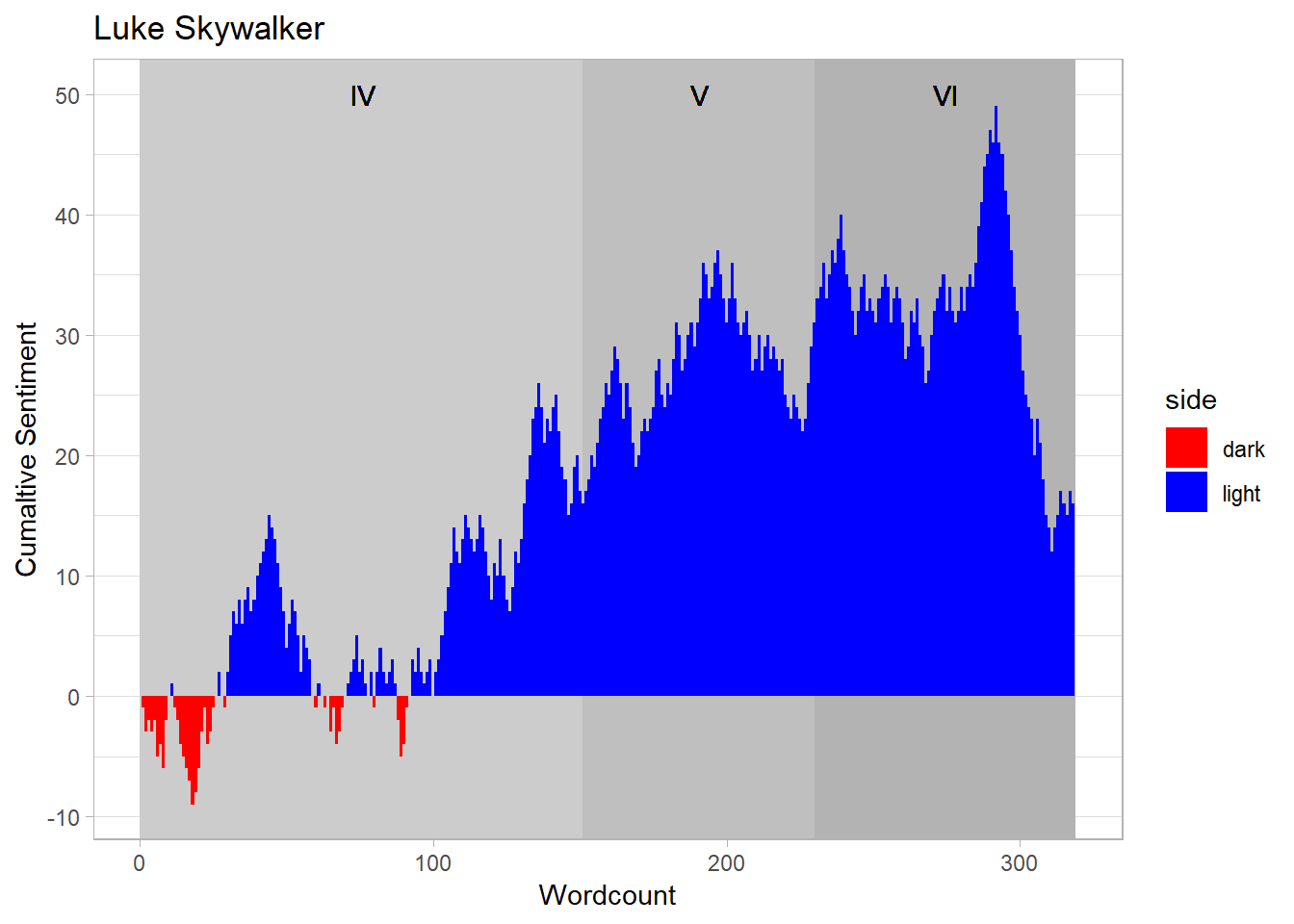
We can see that Luke really struggles at the beginning of A New Hope, which makes sense as his whole world is shattered and his home destroyed very early on in this film. We can see he continues to struggle, but finally ends the film with a fairly sizable chunk of “Light Side Sentiment”. This continues to build up during the other two films and then has a dramatic fall right at the finale. Which again seems intuitive as he finally battles the Emperor and loses his father.
Now let’s contrast this with Dad.
minmax <-
  word_sentiments %>%
  filter(character == "VADER") %>%
  group_by(film) %>%
  summarise(min = min(wordcount),
            max = max(wordcount))

word_sentiments %>%
  filter(character == "VADER") %>%
ggplot() +
  labs(y = "Cumaltive Sentiment", x = "Wordcount", title = "Darth Vader") +
  theme_light() +
  geom_rect(alpha = 0.7, fill = "grey80", aes(xmin = 0, xmax = minmax$max[1], ymin = -Inf, ymax = Inf)) +
  geom_rect(alpha = 0.7, fill = "grey75", aes(xmin = minmax$min[2]-1, xmax = minmax$max[2], ymin = -Inf, ymax = Inf)) +
  geom_rect(alpha = 0.7, fill = "grey70", aes(xmin = minmax$min[3]-1, xmax = minmax$max[3]+1, ymin = -Inf, ymax = Inf)) +
  geom_col(aes(wordcount, cuma_sent, fill = side), width = 1.01) +
  geom_text(aes(x = (minmax$max[1] + minmax$min[1])/2, y = 20), label = "IV") +
  geom_text(aes(x = (minmax$max[2] + minmax$min[2])/2, y = 20), label = "V") +
  geom_text(aes(x = (minmax$max[3] + minmax$min[3])/2, y = 20), label = "VI") +
  scale_fill_manual(values = c("red", "blue"))
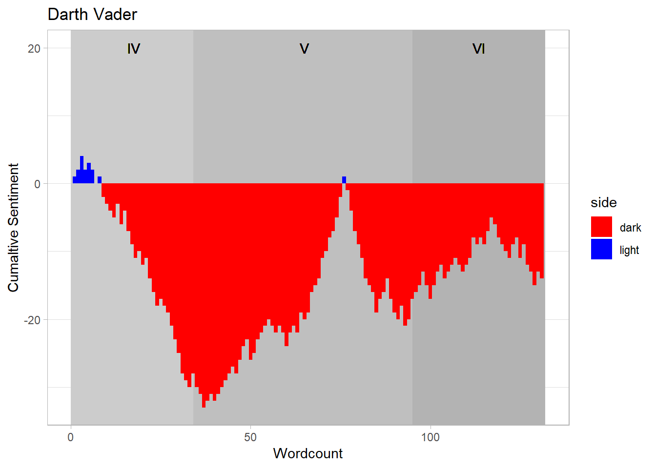
Well it turns out the Darth was a pretty negative guy! Who knew!
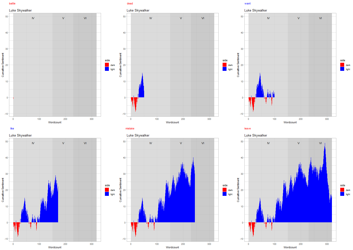
Now the final twist I wanted to get out of this data - can I somehow visualise the words that are causing the fluctuations in sentiment? This is where animation allows us to bring another factor into play. Now this process was a bit of a hack, as I don’t believe it is possible to animate two graphs side by side with gganimate yet. So the process I took was:
Create the first animated bar plot:
minmax <-
  word_sentiments %>%
  filter(character == "LUKE") %>%
  group_by(film) %>%
  summarise(min = min(wordcount),
            max = max(wordcount))

x <-
  word_sentiments %>%
  filter(character == "LUKE") %>%
  ggplot() +
  labs(y = "Cumaltive Sentiment", x = "Wordcount", title = "Luke Skywalker") +
  theme_light() +
  #annotate("rect", xmin = 0, xmax = minmax$max[1], ymin = -Inf, ymax = Inf, alpha = 0.2, fill = "red")
  geom_rect(alpha = 0.7, fill = "grey80", aes(xmin = 0, xmax = minmax$max[1], ymin = -Inf, ymax = Inf)) +
  geom_rect(alpha = 0.7, fill = "grey75", aes(xmin = minmax$min[2]-1, xmax = minmax$max[2], ymin = -Inf, ymax = Inf)) +
  geom_rect(alpha = 0.7, fill = "grey70", aes(xmin = minmax$min[3]-1, xmax = minmax$max[3]+1, ymin = -Inf, ymax = Inf)) +
  geom_col(aes(wordcount, cuma_sent, fill = side), width = 1.01) +
  geom_text(aes(x = (minmax$max[1] + minmax$min[1])/2, y = 50), label = "IV") +
  geom_text(aes(x = (minmax$max[2] + minmax$min[2])/2, y = 50), label = "V") +
  geom_text(aes(x = (minmax$max[3] + minmax$min[3])/2, y = 50), label = "VI") +
  scale_fill_manual(values = c("red", "blue")) +
  transition_states(wordcount, wrap = F) + shadow_mark()

xgif <- animate(x, duration = 36.75, fps = 20)

xgif
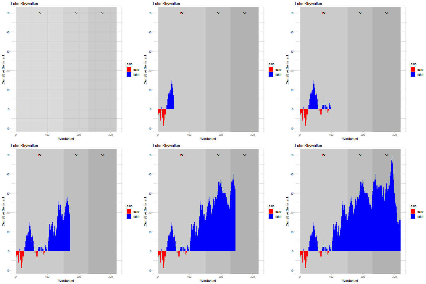
Then animate the words that get scored as below:
 y <-
   word_sentiments %>%
  filter(character == "LUKE") %>%
   ggplot(aes(1,1, colour = word_side)) + geom_text(aes(label = word))  + theme_void() + theme(legend.position = "none") + transition_states(wordcount) + scale_colour_manual(values = c("red", "blue"))

ygif <- animate(y, duration = 36.75, fps = 20)

ygif

Then finally use the magick package to stitch each frame of both the gifs together. This was a painfully slow script to run (and I also cropped my words gif in an online editor), but it does get the result I wanted.
 x_mgif <- image_read(xgif)
 y_mgif <- image_read(ygif)

 new_gif <- image_append(c(y_mgif[1], x_mgif[1]), stack = T)
 for(i in 2:734){
   combined <- image_append(c(y_mgif[i], x_mgif[i]), stack = T)
   new_gif <- c(new_gif, combined)
   print(paste0("combined up to ", i))
 }
After stitching together we finally get the desired result:

As always plenty of experimentation took place beforehand, with my personal favourite fail being the following:
